Robotic Welding for Small Batches: Programming, Changeover and Batch-Size Economics
Small-batch robotic welding becomes attractive when the time saved on each assembly is enough to cover the work needed to prepare that batch. The critical inputs are programming, fixture changeover, first-piece approval and the complete production cycle.
A short weld time alone does not answer the purchasing question. A robot can weld an assembly quickly and still take longer to complete an urgent order because the job has not been programmed or the fixture is unavailable. A repeat order using a proven program and fixture can have a very different result.
Evaluate each part family twice: once as a new job and once as a repeat job. Then separate the production-time decision from the cost decision.
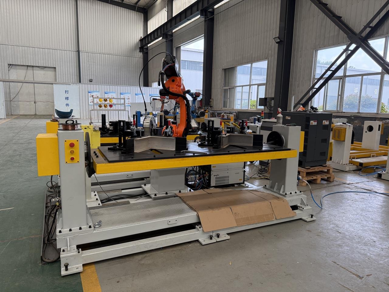
Start with the part family, not the factory’s monthly total
For mixed production, “we weld many hours per month” hides how those hours are distributed. A factory may have one stable repeat assembly and dozens of unrelated repair jobs. Only the repeat assembly may initially justify dedicated robotic tooling.
Group jobs according to what can actually be reused:
- Joint type, welding process and quality requirement.
- Datum scheme, fixture base and change parts.
- Torch access, weld sequence and positioner arrangement.
- Robot program structure and approved parameter sets.
- Material preparation and incoming-part consistency.
Similar-looking parts are not automatically one production family. A new clamp location can obstruct an existing approach path; a changed thickness can require process review.
Use the robot welding cell selection guide to shortlist a cell architecture. Use the batch analysis below to decide which jobs should occupy it.
Keep engineering work separate from recurring changeover
A useful estimate has three cost and time categories.
| Category | Examples | How to account for it |
|---|---|---|
| First-time engineering | Fixture design, initial programming, commissioning and process development | Charge to the new job or spread over a credible repeat-order quantity. |
| Recurring batch setup | Retrieve the correct program, change tooling, confirm references and approve the first piece | Include every time the job is restarted after changeover. |
| Production per assembly | Loading, sensing, welding, repositioning, unloading and routine inspection | Measure the complete repeatable cycle and the labor attention it requires. |
Offline programming can move part of the programming work away from the production cell. It does not make the engineering effort disappear. ABB’s ArcWelding PowerPac description explains how weld paths are generated from CAD geometry. ABB’s training syllabus also includes calibration to the real part and subsequent program adjustment.
For a quotation, distinguish software preparation time from the time needed at the physical cell. Confirm that the robot, software options, tooling model and available programming skills support the proposed workflow.
Define what makes a saved job reusable
A saved robot program is only one part of a repeatable setup. Link it to the drawing revision, fixture and change-part IDs, active tool and workpiece frames, power-source settings, weld sequence and first-piece inspection record. Include any sensing routine and the allowed input-part variation.
Classify changes before estimating reuse. A new order quantity may need only production planning. A different locator or torch neck may require reference checks. A changed joint, material thickness or required weld can require new process development. The job history should show which work is repeatable and which engineering must be done again.
In an illustrative 50-piece repeat order with a 3-minute cycle, an unexpected 45-minute reteach adds 45 ÷ 50 = 0.9 minutes per delivered assembly before considering its specialist labor cost. Calling that intervention “minor” does not remove it from the economics.
Measure the whole cycle and record who is occupied
Separate arc-on time from robot motion, loading, clamping, sensing, positioner movement, torch service and inspection. Miller’s weld-data guide treats arc-on time, defect costs and throughput as related but distinct sources of production information. An arc-on percentage cannot establish accepted output on its own.
For periodic work, allocate its observed time across the units between events. If an illustrative 90-second service event is required every 30 assemblies, it contributes 3 seconds per assembly. Include unplanned stops separately. Do not add the allocation again if the timed production average already contains those events.
Record labor by person and activity. If an operator loads another station while the robot welds, the robot and labor clocks overlap. If the operator must stay available throughout the cycle, charging only the seconds spent touching the part may understate the staffing requirement. Record both hands-on work and the staffing arrangement necessary to sustain the output.
First calculate when the batch becomes faster
The following is an illustrative planning example, not a HORISTAR production result. Assume the same acceptable weld outcome for both routes, no rejected parts and a sequential single-station cycle.
| Time input | Manual route | Robot route |
|---|---|---|
| Recurring setup and first-piece approval | 15 minutes | 60 minutes |
| Complete production cycle per assembly | 7 minutes | 3 minutes |
Let N be the number of assemblies:
- Manual batch time =
15 + 7 × Nminutes. - Robot batch time =
60 + 3 × Nminutes.
The robot recovers its additional 45 minutes of setup by saving 4 minutes per assembly:
Time crossover = (60 − 15) ÷ (7 − 3) = 11.25 assemblies.
Under these assumptions, the robot route becomes faster at 12 assemblies. At 12 pieces, manual production takes 99 minutes and robotic production takes 96 minutes. That is a small difference; a short delay in first-piece approval could reverse it.
| Batch size | Manual elapsed time | Robot elapsed time | Time result |
|---|---|---|---|
| 8 | 71 minutes | 84 minutes | Manual finishes sooner. |
| 12 | 99 minutes | 96 minutes | Robot is only slightly faster. |
| 32 | 239 minutes | 156 minutes | Robot has a clearer time advantage. |
| 50 | 365 minutes | 210 minutes | Robot saves 155 minutes. |
This comparison assumes both resources are ready when the order arrives. Add queue time when delivery is the objective. A robot waiting for a programmer may finish later than an available manual station even when its processing time is lower.
For dual-station systems, measure elapsed output directly. Loading and welding may overlap, so adding every activity duration can overstate the cycle. Record operator attendance separately from machine elapsed time.
For an idealized alternating two-station cell, the steady-state interval can be estimated as:
Output interval ≈ longer of robot-side time and operator-side time + non-overlapping exchange time.
If those illustrative times are 3.0, 2.0 and 0.3 minutes, the interval is 3.3 minutes, giving about 18.2 assemblies per hour before other losses. If loading and required inspection increase to 4.0 minutes, the interval becomes 4.3 minutes, or about 14.0 per hour. A faster weld then provides no benefit until the longer operator-side task is reduced.
This model assumes the tasks can actually overlap, one assembly is completed per exchange, and there is no additional waiting beyond the longer modeled task. A short batch also includes the initial fill and final emptying of the cell. Verify those boundaries from a timeline; do not multiply a steady-state rate by a few minutes and treat it as a complete batch forecast.
Then calculate when the batch costs less
Use cost inputs that match the decision. For a repeat order on an existing cell, estimate the relevant setup and production costs. For a new equipment purchase, also examine ownership cost, utilization and the number of repeat orders that will actually occur.
Continue with a separate set of illustrative cost assumptions:
| Cost input | Manual route | Robot route |
|---|---|---|
| Recurring setup cost per batch | USD 12 | USD 60 |
| Recurring cost per acceptable assembly | USD 4.00 | USD 2.50 |
The unit costs can be built from the earlier cycle times with the following illustrative rate assumptions. These are calculation inputs, not market rates or a quotation.
| Recurring unit-cost component | Manual route | Robot route |
|---|---|---|
| Labor at USD 24/hour | 7.0 attended minutes = USD 2.80 | 1.2 allocated attended minutes = USD 0.48 |
| Equipment at USD 3/hour manual and USD 30/hour robot | 7.0 minutes = USD 0.35 | 3.0 minutes = USD 1.50 |
| Consumables and other variable process costs | USD 0.85 | USD 0.52 |
| Total per assembly, with no rejects | USD 4.00 | USD 2.50 |
Equipment rates here exclude all separately listed labor and variable process costs. The robot labor allocation assumes the remaining operator time is productively shared; use the full required staffing cost if that assumption does not hold.
For setup, the manual example allocates 15 minutes at USD 27/hour for labor plus equipment, and USD 5.25 for setup-specific supplies and tooling allocation: USD 12 total. The robot allocates 60 minutes at USD 54/hour plus USD 6 for setup-specific supplies: USD 60 total. First-piece approval is included in the setup interval. Keep any program engineering or tooling investment outside those recurring figures unless it actually recurs.
The model excludes the common value of the incoming assembly from both routes while yield is 100%. The loss of that assembly becomes important when rejects are introduced below.
The batch costs are:
- Manual cost =
12 + 4.00 × N. - Robot cost =
60 + 2.50 × N.
Cost crossover = (60 − 12) ÷ (4.00 − 2.50) = 32 assemblies.
At 32 assemblies, both routes cost USD 140. Above 32, the robot route is less expensive under this model. At 50 pieces, the manual route costs USD 212 and the robot route costs USD 185.
The same example therefore gives two different answers:
- At 12 pieces, the robot is slightly faster but costs USD 90 versus USD 60.
- At 50 pieces, it is both faster and less expensive.
That distinction helps production and purchasing discuss a rush order without confusing delivery value with manufacturing cost.
What happens on the first order?
Suppose the robotic route also requires USD 180 of additional first-time engineering, with no corresponding extra manual engineering cost in this example.
For that first batch:
First-order cost crossover = (60 + 180 − 12) ÷ (4.00 − 2.50) = 152 assemblies.
A repeat order can return to the 32-piece crossover only if the program, tooling and process remain reusable. If the design changes, some engineering cost returns.
Repeat orders also retain their recurring setup cost. Ten small orders should not be treated as one large batch when each order needs a separate changeover.
Read the crossover correctly
For a simple comparison:
Cost crossover quantity = additional setup cost ÷ recurring saving per acceptable assembly.
This expression is useful only when the recurring saving is positive. If robotic production costs as much or more per acceptable assembly and also has a higher setup cost, increasing the batch size does not create a cost advantage within that model.
If the robot has both lower setup cost and lower unit cost, there may be no positive crossover to wait for. Check that the supposed setup reduction comes from a demonstrated repeat-job process rather than an omitted activity.
If the robot has lower setup cost but higher unit cost, the direction reverses: it may be cheaper for a small batch and more expensive as quantity grows. Compare the two total-cost expressions instead of treating every crossover as a minimum batch size.
When actual trials produce rejects, replace optimistic cycle averages with the full cost divided by the accepted output. Include rework and replacement production. Keep the inspection standard the same for both routes.
A shorter operator attendance time is also not automatically a payroll saving. Record whether the released time can be used on another productive task. For the investment decision, distinguish additional capacity from cash that will actually leave the cost base.
Recalculate the batch when seam search adds time
Continue the base example at 100% yield, leaving setup unchanged. Suppose a search pattern of eight touches takes 32 seconds per assembly, as in the companion seam-sensing article. Assume the original 3-minute robot cycle excludes this search and that the extra machine time cannot overlap other work.
Keep full precision until selecting the first whole-number batch that wins:
| Result | Calculation | Interpretation |
|---|---|---|
| Robot cycle | 3 + 32 ÷ 60 = 3.533333... min | Search is charged once. |
| Time crossover | 45 ÷ (7 − 3 − 32 ÷ 60) ≈ 12.9808 | Robot faster from 13 assemblies, rather than 12. |
| Robot unit cost | 0.48 + (3 + 32 ÷ 60) × 30 ÷ 60 + 0.52 = USD 2.766666... | Same attended labor and consumables, more equipment time. |
| Cost crossover | 48 ÷ [4 − (0.48 + (3 + 32 ÷ 60) × 30 ÷ 60 + 0.52)] ≈ 38.9189 | Robot cheaper from 39 assemblies, rather than 33. |
Rounding the unit cost to USD 2.77 before calculating the crossover would move the answer to 40 assemblies. Display rounded money for readability, but use the original inputs for the decision.
The unchanged labor line assumes automatic search adds no attended time. If the operator must attend for all 32 additional seconds, labor adds 32 ÷ 60 × 24 ÷ 60 ≈ USD 0.2133 per assembly. Unit cost then becomes USD 2.98, and the cost crossover rises to 48 ÷ (4 − 2.98) ≈ 47.06: cheaper from 48 assemblies. This extra attendance must also fit the operator’s schedule; it cannot simultaneously be credited to another productive task.
This comparison shows what a faster search would have to save. It does not establish that optical sensing pays for itself. Compare the measured cycle and quality benefit with its added hardware, integration, support and training costs.
Stress-test the result against yield and the value of a scrapped assembly
Dividing welding cost by first-pass yield can understate a failure’s cost when welding occurs after expensive cutting, bending or machining. A rejected weld may destroy the value already in the assembly.
For a simplified scrap-only planning model, define:
q: accepted fraction of attempted assemblies, with no recovery by rework.c: recurring welding and inspection cost per attempt.v: incoming assembly value lost on each scrapped attempt, net of salvage.
The incremental cost per accepted assembly is:
c_good = [c + (1 − q) × v] ÷ q.
The ordinary incoming value of the accepted assembly is omitted because it is common to both routes. The extra lost value is included. The model assumes stable yield across attempts; it estimates expected cost, not a guarantee that a small batch will produce an exact number of good parts.
Hold the manual route at the earlier illustrative USD 4.00 per good assembly and 100% yield. For the robot use c = USD 2.50, v = USD 12, and the same USD 48 additional recurring setup cost:
| Assumed robot yield | Robot cost per accepted assembly | Repeat-batch cost result |
|---|---|---|
| 100% | USD 2.50 | Equal cost at 32; robot cheaper from 33 parts. |
| 98% | USD 2.80, rounded | Crossover about 39.86; robot cheaper from 40 parts. |
| 95% | USD 3.26, rounded | Crossover about 65.14; robot cheaper from 66 parts. |
| 90% | USD 4.11, rounded | No cost crossover: recurring cost and setup are both higher. |
For the 95% row, [2.50 + 0.05 × 12] ÷ 0.95 ≈ USD 3.2632. Using the unrounded unit cost, 48 ÷ [4.00 − (2.50 + 0.05 × 12) ÷ 0.95] ≈ 65.14. The thresholds are results of these assumptions, not recommended minimum order quantities.
If defects can be repaired, track first-pass acceptance, repair attempts, recovery after repair and final scrap separately. Use total initial production cost, repair cost and net scrap loss divided by final accepted output. Do not divide by first-pass yield after already charging all observed repair and replacement costs; that counts some losses twice.
This is also why the manual and robot trials need the same weld acceptance standard. A route with less inspection can appear cheaper by leaving failures undiscovered.
Check whether the hourly machine rate assumes work that does not exist
A quote can make the robot unit cost look attractive by spreading annual ownership cost over an unrealistic number of loaded hours. For a planning allocation, use:
Machine cost per loaded hour = annual fixed cell cost ÷ realistic loaded hours + variable cost per loaded hour.
Suppose, illustratively, that fixed cell cost is USD 24,000 per year and the separately defined variable machine cost is USD 18 per loaded hour. At 2,000 loaded hours, the rate is USD 30/hour, matching the base example. At 1,000 hours, it is USD 42/hour. Three machine minutes then cost USD 2.10 instead of USD 1.50; total robot unit cost becomes USD 3.10 before rejects.
The higher machine rate also applies to the one-hour robot setup. Its cost rises from USD 60 to USD 72; manual setup remains USD 12. The repeat-batch crossover therefore becomes (72 − 12) ÷ (4.00 − 3.10) ≈ 66.67, so the robot becomes cheaper from 67 parts. Updating the unit cost while leaving the setup rate unchanged would understate this effect.
A batch can be physically identical and have a different allocated cost because the annual business case changed.
Define the denominator consistently. Loaded hours are not automatically all paid shift hours. Deduct planned non-production time and separately model setup, maintenance, material shortages and other losses according to the chosen accounting boundary. If downtime is already reflected in the loaded-hour rate or observed unit cycle, do not add the same downtime factor again.
For dispatching work onto an already owned, otherwise idle cell, the relevant avoidable cost can differ from its fully allocated rate. For deciding whether to buy the cell, include the ownership and support burden. Keep those two questions separate rather than using whichever rate produces the preferred result.
Keep investment cash flow separate from allocated job cost
The USD 24,000 annual fixed-cost example is an allocation, not a defined cash-flow statement. Its composition matters. Depreciation or another capital-recovery allocation should not be deducted as a cash operating expense while the same capital purchase is also counted as the initial investment. Actual maintenance payments, software subscriptions and other cash support costs still belong in the relevant period, even when accounting calls them fixed.
Build a separate investment worksheet with the incremental purchase, installation, fixture, integration and training outlay; subsequent cash operating changes; and any residual proceeds under the chosen analysis. Count labor cash savings only when payroll, overtime or purchased labor actually falls. If people are reassigned, identify additional saleable output and its net contribution instead of also counting the same hours as payroll savings.
For a basic, undiscounted screening calculation with constant positive annual net cash benefit, simple payback = incremental initial outlay ÷ annual net cash benefit. Changing annual benefits need a year-by-year cumulative calculation. Simple payback leaves out the time value of money and later returns; the U.S. Department of Energy’s discussion of payback also notes its limited view of continuing benefits.
Use consistently allocated costs for the stated job-cost comparison, relevant avoidable costs and capacity constraints for a dispatch decision, and incremental cash flows for the investment. The USD 27 saving on a 50-piece order is not automatically USD 27 of cash available to recover a cell purchase.
Count separate setups when forecasting repeat demand
Using the original 100%-yield assumptions, an illustrative total demand of 200 assemblies produces very different annual totals depending on its release pattern:
| Release pattern | Manual recurring cost | Robot recurring cost |
|---|---|---|
| 20 batches of 10 | 20 × 12 + 200 × 4 = USD 1,040 | 20 × 60 + 200 × 2.5 = USD 1,700 |
| 2 batches of 100 | 2 × 12 + 200 × 4 = USD 824 | 2 × 60 + 200 × 2.5 = USD 620 |
The same 200 pieces can favor either route. Combining orders helps only if delivery dates, revisions, storage and inventory commitments permit it. Producing uncertain future demand early is not a free setup reduction.
For a part family with quantities N₁ ... Nₘ over m separate batches, estimate total robot cost as initial engineering plus m × setup cost plus the sum of each batch’s accepted-output cost. Evaluate the low, expected and high repeat-demand cases using actual order history or an explicitly uncertain forecast.
In the base example, a 50-piece repeat order saves USD 27. Seven such orders save USD 189, enough to recover the illustrative USD 180 additional engineering cost if nothing changes. That is recovery of one job’s engineering expense; it does not establish payback of the entire robotic cell.
Reduce changeover by finding its largest component
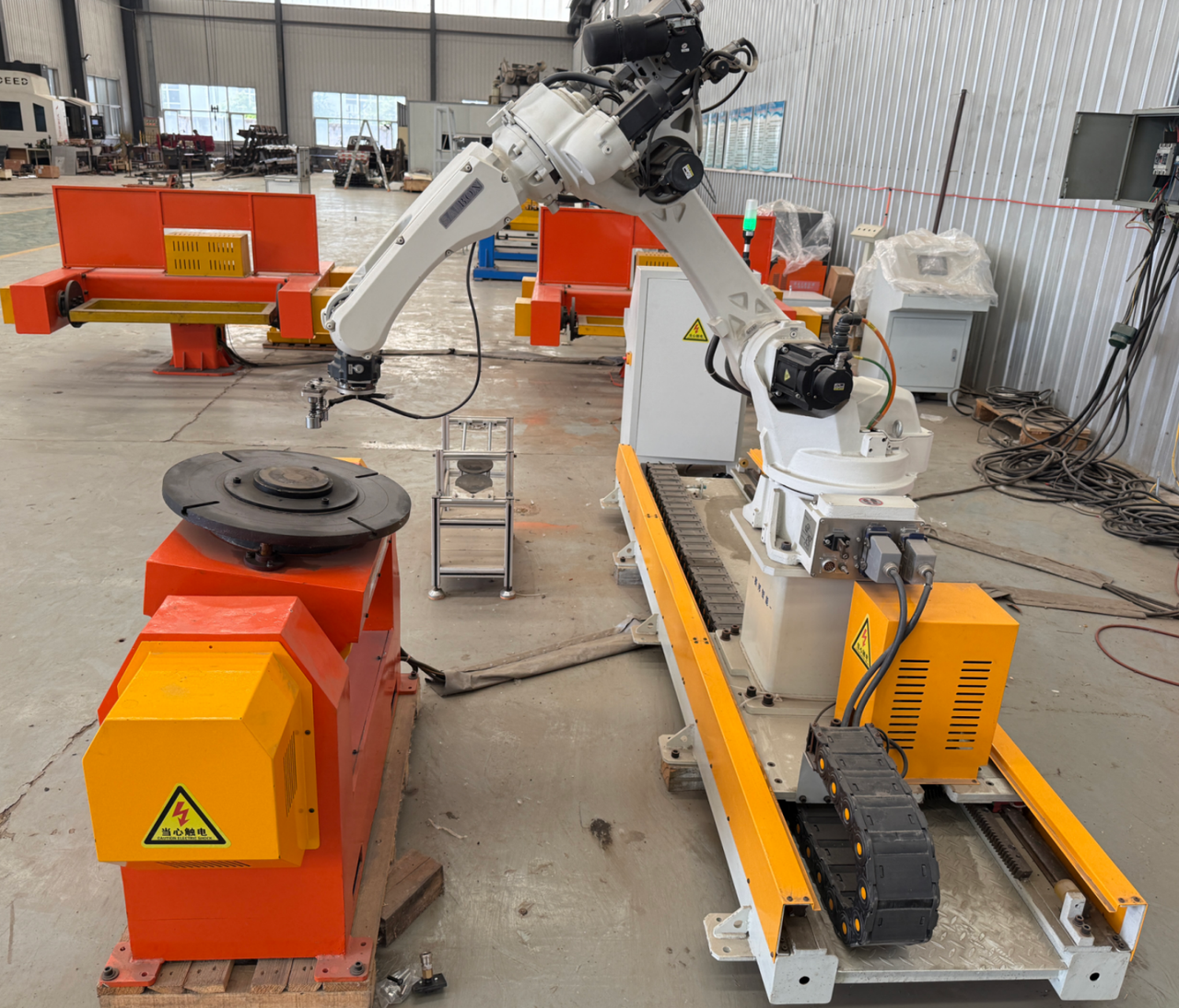
Time one complete change from the last acceptable part of Job A to the first approved production part of Job B. Record concurrent activities as concurrent; the elapsed changeover is not necessarily their sum.
Use this worksheet during the observation:
| Activity | Start/end or duration | Cell stopped? | Person required | Main cause of delay | Proposed change |
|---|---|---|---|---|---|
| Obtain the correct program and revision | — | — | — | — | — |
| Retrieve and install fixture change parts | — | — | — | — | — |
| Load parts and confirm seating | — | — | — | — | — |
| Confirm references and run the approved path check | — | — | — | — | — |
| Produce and inspect the first piece | — | — | — | — | — |
| Make corrections and release production | — | — | — | — | — |
The pattern determines the improvement:
- Program retrieval dominates: improve revision control and job identification before buying faster programming software.
- Tooling retrieval dominates: prepare labeled change parts while the previous job runs, where the cell’s approved workflow permits it.
- Physical adjustment dominates: investigate locator repeatability and controlled settings.
- First-piece rejection dominates: address incoming-part variation or the welding process before shortening inspection.
- Offline work dominates: assess whether CAD preparation and reusable program structures reduce the engineering burden.
The fixture inspection guide is useful when repeated adjustment originates in seating, clamp direction or uncontrolled change parts.
Moving work outside the stopped-cell interval changes time and cost differently
The Lean Enterprise Institute’s SMED explanation distinguishes setup that requires a stopped machine from preparation possible while it runs. Use that distinction to examine the observed changeover, without promising that every activity can be moved.
Suppose, illustratively, 25 of the original 60 robot setup minutes can be completed before the job starts: preparing change parts, checking program revisions and organizing inspection documents. Internal setup becomes 35 minutes. This assumes preparation does not interrupt the preceding job, create another labor bottleneck or delay this order.
The time crossover becomes (35 − 15) ÷ (7 − 3) = 5 assemblies. The routes finish together at five, and the robot finishes sooner from six. Preparation time still exists; it has moved outside this batch’s stopped-cell interval.
Keep its labor in the cost:
| Robot setup component | Illustrative cost |
|---|---|
| 35 internal minutes at USD 54/hour | USD 31.50 |
| 25 external minutes at USD 24/hour | USD 10.00 |
| Setup-specific supplies | USD 6.00 |
| Total robot setup cost | USD 47.50 |
With the original USD 12 manual setup and USD 1.50 recurring unit saving, the cost crossover is (47.50 − 12) ÷ 1.50 ≈ 23.67: the robot is cheaper from 24 assemblies.
Stopped-cell time falls by 25 minutes, but the 60 total labor minutes remain. The USD 12.50 reduction in allocated setup cost is 25 ÷ 60 × USD 30/hour of released cell time. It is not automatically a cash saving: the fixed portion of that rate may continue, and the value of available capacity depends on other work. Record delivery improvement, capacity released and avoidable cash cost separately.
This example and the search-time example vary different inputs independently. If both changes occur, combine the 35-minute internal setup, USD 47.50 setup cost and the measured revised unit cycle in one model; do not add their separate crossover reductions.
Run a repeat-order trial, not just a first demonstration

A supplier demonstration may begin with the fixture already installed and the program ready. That is useful cycle evidence, but it leaves changeover unmeasured.
For a more relevant trial, propose the sequence A → B → A using two representative part families. Under the agreed safe operating procedure, record:
- The complete setup, first-piece approval and production time for A.
- The change to B, including tooling and program verification.
- The return to A using the saved setup.
- Accepted output, rework, operator attendance and any specialist intervention.
The return to A tests whether the claimed repeat-order advantage is reproducible. If a programmer must reteach several positions each time, include that work in the recurring estimate until the cause is resolved.
Agree what the buyer’s normal operator must be able to do after training. A cycle achievable only with the supplier’s specialist standing beside the cell may not represent daily production.
Decide which jobs to automate first
Start with families that combine repeat demand, stable revisions, practical fixturing and enough recurring savings to recover setup. Keep uncertain prototypes and frequently redesigned work in a separate estimate.
For a HORISTAR robotic welding enquiry, send drawings, material and joint details, batch sizes by part family, repeat-order frequency, current cycle times and the observed changeover record. Ask for the proposed programming route and a trial that includes changing away from and back to the same job.
The result should be a job-level decision: which orders fit the cell now, which need a better changeover process, and which remain more practical through another production route.